YIMBies Overpromise
--Intro
--Data
--Core Data
--Expanded Data
--Storytelling
--Regressions
--A tale of two cities
--Nightmares
Intro
Alright, so people seem to dig really deep data dives onto controversial subjects so...YIMBYism.
The main thing I'm interested in here is less "Does YIMBYism work" and more...how much construction is actually needed to achieve YIMBY goals? Like, pretend you're appointed the Supreme Mega Dictator for San Francisco, you've got unlimited legal and extralegal authority, how much construction would it actually take to drop rental prices by 30%? Is that actually a thing, like has some city in the US actually managed to build so much housing that prices didn't just drop but dropped significantly? If so, what did they do?
'Cuz at some point, somebody actually has to do this, some mayor or county official or somebody actually has to execute real policy and that policy needs to actually have a real effect. Somebody has to lay out a realistic path, pointing to things other people have done in the past, to achieving significant reductions in rental and housing prices because, well, I know a lot of people laugh at people in SF and NY and these places for spending absurd amounts of money on housing but...when it's your friends and family, it really sucks.
As for why me...well, I'm really ignorant. No, seriously, I've got technical skills, there's going to be a lot of R code in this post, but I don't really have much understanding of the housing market. And if you want fresh insights and fresh perspectives on a subject, you kind of need ignorance, you need somebody who doesn't know the obvious stuff. So that's the core pitch, you can't "hurr, durr you no understand economics" 'cuz I'm going to go fairly deep into the data but hopefully I'll find some new stuff via bringing a new perspective. And yeah, no references, no links by and large, just raw data and my data analysis.
Speaking of code, I'm going to try intermixing code with analytics this time and we're going to try doing it in R's tidy style. I think the analysis is going to be simple enough to mix in to the article and the tidyr style is simple enough that lay people might be able to understand what the code is doing. We'll see how it works, let me know if you super digg or or hate it in the comments; I'm trying the tidy style because of a comment someone left last time.
Core Data
The big thing that got this started is data, specifically AEI's "New Construction Data". I mean, Zillow has great data and makes most of it available but they don't actually have and/or share information on new housing construction. And while you might think there's a nice national database of new housing construction, to the best of my knowledge there isn't, it's all locked away in, like, county assessors offices and stuff. Lots of the housing and rental prices were similarly locked away in local MLS...es until Zillow showed up. And AEI has taken the Zillow dataset and then went and done the yeoman work of getting as many housing construction records as possible and putting them together with Zillow housing data. So there's actually a nice clean data set with all the housing construction and price data for the US, not just at the metro city level but also for tens of thousands of individual zip codes. And once you see a nice clean data set like that, man, the analysis is easy, they've already done the hard work.
So applause to AEI. This is exactly the sort of thing that should be encouraged and making large, clean data sets like this is super helpful and important.
Expanded Data
So we could do a lot of fancy analysis to try to figure out what kinds of variables we have but the AEI guys actually wrote really nice documentation, which you can read here: https://www.aei.org/wp-content/uploads/2021/01/AEI-Zillow-New-Construction-Sales-Index-Methodology-Codebook-v6-clean.pdf?x91208.
require(tidyr)
require(magrittr)
require(dplyr)
require(ggplot2)

raw_df<-read.csv("https://www.aei.org/wp-content/uploads/2023/04/aei_zillow_new_c_data_2022Q4.csv"
                 , stringsAsFactors = F)

df<-raw_df %>%
  select(cbsa_short, orig_y, price_new_c, count_weighted, new_c) %>%
  rename(Metro_Area=cbsa_short, year=orig_y
         , Median_Price=price_new_c, New_Construction=count_weighted
         , New_Construction_Percent_Sales=new_c) %>%
  mutate(year=as.character(year)) %>%
  filter(Metro_Area != "National") %>%
  filter(Metro_Area != "") %>%
  na.omit()

output_df<-df %>%
  group_by(Metro_Area, year) %>%
  summarise(total_new_construction=sum(New_Construction)
            , avg_percent_sales_new_construction=mean(New_Construction_Percent_Sales)
            , avg_price=mean(Median_Price))


filter(output_df, Metro_Area=="San Francisco, CA")
This should give you a good idea of the data we're working with. The underlying data is a lot more granular, breaking it down by subregions and price tiers but we're just simplifying that data for reasons that will become apparent soon. So we've got San Francisco, from 2012-2022, and the total number of new constructions, the percent of total real estate sales involving new construction, and the median price for the new construction. So, for example, in 2016, San Francisco sold 3,930 newly constructed properties for an average price of $1,157,000 dollars. These newly constructed properties were about 17% of all sales, so we can extrapolate roughly ~23,000 properties were sold.
But here's where I want to expand on this original data in a few interesting ways. I love the construction data but let's expand on that using three different data sets.
First, the price data we reference here is...not ideal. Simply, the original price data is median sale price for new construction for very granular areas,think like individual zip codes. If we try to just take the mean of all that data, it gets funky. Instead, let's just go grab the Zillow data for the whole city, which will also give us sale price for all properties, not just new construction, and rental data. So, running off the Zillow data, in the San Francisco MSA (so also Oakland, Fremont, etc) the average property sold for ~$668k and the average rent was $2,628.
Second, let's go grab some inflation data from FRED so we can do calculations in inflation adjusted dollars. Especially with recent inflation, we're looking at an overall 30% price change, or a $100k house in 2012 being equivalent price to a $130k house in 2022. That'll let us work of real prices, rather than nominal ones.
Finally, let's work off population rather than percent of homes sold. I know what AEI was going for with the percent new construction, and I do like it but...I think new construction vs population is closer match to what people are looking for. So, for example, in 2016, San Francisco built 3930 new properties. This was 17% of all real estate sales. At the same time, the population for San Francisco increased by 24,233 people, so, roughly, SF built ~4k homes for ~24k new people or 1 property for every six new residents. I like the first statistic that AEI provides...but I think that second one is better.
#Data to parse in
#https://www.zillow.com/research/data/
#These links will probably change
#Zillow-Median Sale Price (Smooth, All Homes, Monthly)-Metro & US
Sales_raw<-read.csv("https://files.zillowstatic.com/research/public_csvs/median_sale_price/Metro_median_sale_price_uc_sfrcondo_sm_month.csv?t=1688350084", stringsAsFactors = F)

#Zillow-ZORI (Smoothed): All Homes Plus Multifamily Times Series ($)-Metro & US
Rent_raw<-read.csv("https://files.zillowstatic.com/research/public_csvs/zori/Metro_zori_sm_month.csv?t=1688350084", stringsAsFactors = F)
Sales<-Sales_raw %>%
  filter(RegionType=="msa") %>%
  filter(RegionName %in% df$Metro_Area) %>%
  select(!(c(RegionID, SizeRank, RegionType, StateName))) %>%
  pivot_longer(
    cols=starts_with("X")
    , names_to="year"
    , values_to = "Median_Sale_Price"
  ) %>%
  mutate(across(c('year'), substr, 2, 5)) %>%
  rename(Metro_Area=RegionName, year=year, Median_Sale_Price=Median_Sale_Price) %>%
  group_by(Metro_Area, year) %>%
  summarise(Average_Sale_Price=mean(Median_Sale_Price))

Rent<-Rent_raw %>%
  filter(RegionType=="msa") %>%
  filter(RegionName %in% df$Metro_Area) %>%
  select(!(c(RegionID, SizeRank, RegionType, StateName))) %>%
  pivot_longer(
    cols=starts_with("X")
    , names_to="year"
    , values_to = "Avg_Rent"
  ) %>%
  mutate(across(c('year'), substr, 2, 5)) %>%
  rename(Metro_Area=RegionName, year=year, Avg_Rent=Avg_Rent) %>%
  group_by(Metro_Area, year) %>%
  summarise(Avg_Rent=mean(Avg_Rent, na.rm=TRUE))

#https://fred.stlouisfed.org/series/FPCPITOTLZGUSA
inflation_data<-data.frame(
  year=c("2012", "2013", "2014", "2015", "2016", "2017", "2018", "2019", "2020", "2021", "2022")
 , inflation_rate=c(1.0206, 1.0146, 1.0162, 1.0011, 1.0126, 1.0213, 1.0244, 1.0181, 1.0123, 1.0469, 1.0800))
cumulative_inflation<-c()
for (i in 1:nrow(inflation_data)){
  cumulative_inflation<-c(cumulative_inflation
  ,ifelse(
     inflation_data$year[i]=="2012", inflation_data$inflation_rate[i]                                                                                                                  , inflation_data$inflation_rate[i]*cumulative_inflation[i-1]))
}
inflation_data<-cbind(inflation_data, cumulative_inflation)

#https://www.census.gov/data/datasets/time-series/demo/popest/2010s-total-metro-and-micro-statistical-areas.html
#https://www.census.gov/data/datasets/time-series/demo/popest/2020s-total-metro-and-micro-statistical-areas.html
old_census<-read.csv("your local file here", stringsAsFactors = F)
new_census<-read.csv("your local file here", stringsAsFactors = F)
old_census$MSA<-substring(old_census$MSA, 2 , (nchar(old_census$MSA)-11))
old_census<-old_census %>%
  pivot_longer(cols=starts_with("X")
               , names_to="year"
               , names_prefix="X"
               , values_to="Population") %>%
  rename(Metro_Area="MSA")
old_census$Population<-gsub(",", "", old_census$Population)
old_census$Population<-as.integer(old_census$Population)
new_census<-new_census %>%
  filter(LSAD=="Metropolitan Statistical Area") %>%
  select(NAME, POPESTIMATE2020, POPESTIMATE2021, POPESTIMATE2022) %>%
  rename(Metro_Area="NAME", P2020="POPESTIMATE2020", P2021="POPESTIMATE2021"
         , P2022="POPESTIMATE2022") %>%
  pivot_longer(cols=starts_with("P")
               , names_to="year"
               , names_prefix=("P")
               , values_to="Population")
census<-rbind(old_census, new_census)
#Uggh, lot of name mismatches
#Alright, core issue is there's lot's of dash stuff, like Chicago-Naperville-Elgin, IL-IN-WI
#So, split the string on comma so we have city then state
#then grab everything before the first "-" for each, then repaste
for (i in 1:nrow(census)) {
  raw<-unlist(strsplit(census$Metro_Area[i], ","))
  city<-raw[1]
  state<-raw[2]
  city<-unlist(strsplit(city, "-"))[1]
  state<-unlist(strsplit(state, "-"))[1]
  census$Metro_Area[i]<-paste(city, state, sep=",")
}
#And two quick manual patches
census$Metro_Area[census$Metro_Area=="Louisville/Jefferson County, KY"]<-"Louisville, KY"
census$Metro_Area[census$Metro_Area=="Riverside, CA"]<-"Riverside_SB, CA"
#Quick Check
master_df<-output_df %>%
  left_join(Sales
            , by=join_by(Metro_Area, year)) %>%
  left_join(Rent
            , by=join_by(Metro_Area, year)) %>%
  left_join(inflation_data
            , by=join_by(year)) %>%
  left_join(census
            , by=join_by(Metro_Area, year))
  #there are 75 na values, like we don't have rental price data for Akron, Ohio in 2012
master_df<-master_df %>%
  mutate(absolute_pop_change=Population-lag(Population)
         , percent_pop_change=Population/lag(Population)
         , real_sale_price=Average_Sale_Price/cumulative_inflation
         , real_rent=Avg_Rent/cumulative_inflation)
City Analysis
Alright, let's start by analyzing cities. What cities has the smallest price and rent growth?
bottom_line_df_nominal<-master_df %>%
  select(Metro_Area, year, Average_Sale_Price , Avg_Rent) %>%
  filter(year<2020) %>%
  arrange(Metro_Area, year) %>%
  mutate(sale_price_change=Average_Sale_Price/lag(Average_Sale_Price)
         , rent_change=Avg_Rent/lag(Avg_Rent)) %>%
  group_by(Metro_Area) %>%
  summarise(price_change=mean(sale_price_change, na.rm=T)
            , rent_change=mean(rent_change, na.rm=T))

bottom_line_df_real<-master_df %>%
  select(Metro_Area, year, real_sale_price, real_rent) %>%
  filter(year<2020) %>%
  arrange(Metro_Area, year) %>%
  mutate(real_sale_price_change=real_sale_price/lag(real_sale_price)
         , real_rent_change=real_rent/lag(real_rent)) %>%
  group_by(Metro_Area) %>%
  summarise(price_change=mean(real_sale_price_change, na.rm=T)
            , rent_change=mean(real_rent_change, na.rm=T))

bottom_line_df_nominal %>%
  arrange(price_change) %>%
  select(Metro_Area, price_change) %>%
  rename("Metro Area"=Metro_Area
         , "Average Annual Housing Price Change, Nominal"=price_change) %>%
  slice_head(n=10)

bottom_line_df_nominal %>%
  arrange(rent_change) %>%
  select(Metro_Area, rent_change) %>%
  rename("Metro Area"=Metro_Area
         , "Average Annual Rental Price Change, Nominal"=rent_change) %>%
  slice_head(n=10)
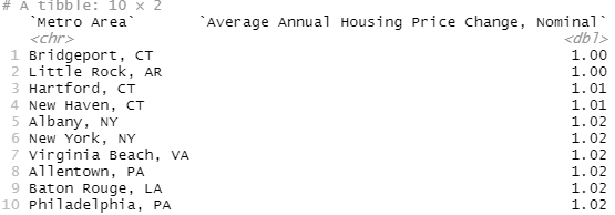
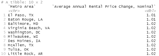
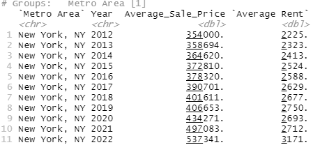
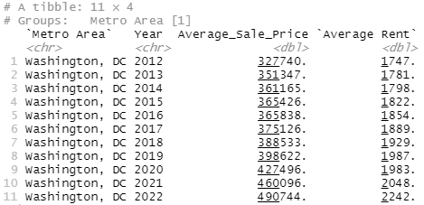
Wait, what? Wait, wait, wait, what? New York, New York of, well, New York fame has the one of the lowest annual housing price increases on Zillow? And Washington DC has some of the lowest rental growth in the nation?!? This, uh, this does not match my preconceived notions.
bottom_line_df_real %>%
  arrange(price_change) %>%
  select(Metro_Area, price_change) %>%
  rename("Metro Area"=Metro_Area
         , "Average Annual Housing Price Change, Real"=price_change) %>%
  slice_head(n=10)

bottom_line_df_real %>%
  arrange(rent_change) %>%
  select(Metro_Area, rent_change) %>%
  rename("Metro Area"=Metro_Area
         , "Average Annual Rental Price Change, Real"=rent_change) %>%
  slice_head(n=10)
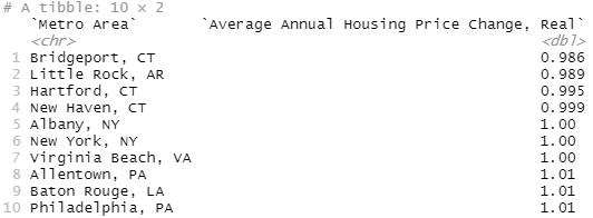
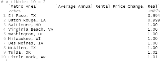
I mean, there's a story here that's important, almost no city in the US has achieved real decreases in price or rental rates and those that have...don't really have high levels of growth so they're not really applicable. But, uh, that NY and DC thing still freak me out. And I'll give you a hint, this isn't a covid thing, I already filtered out the years after 2019. I'll give you a hint, including Covid takes NY off this list but moves Washington DC way off it.
Let's, uh, let's go double check some numbers. I've probably made a mistake. Let's go manually calculate some values for NY and DC and check them.
master_df %>%
  filter(Metro_Area=="New York, NY") %>%
  select(Metro_Area, year, Average_Sale_Price, Avg_Rent) %>%
  rename("Metro Area"=Metro_Area, "Year"=year
         , "Average Rent"=Avg_Rent)

master_df %>%
  filter(Metro_Area=="Washington, DC") %>%
  select(Metro_Area, year, Average_Sale_Price, Avg_Rent) %>%
  rename("Metro Area"=Metro_Area, "Year"=year
         , "Average Rent"=Avg_Rent)
Alright, so manually calculating this in Excel from the Zillow ZORI (rental) data,
NY had an average rent of
2013=$2,323.43
2018=$2,676.61
, while Washington DC had an average rent of
2013=$1,781.38
2018=$1,928.87
For housing, NY has:
2013=$358k
2018=$402k
DC has:
2013=$352k
2018=$388k
Uh, those looks accurate and just looking at the general pricing info, that seems...not what I was expecting. I think this is an MSA thing. Like, we see New York but the New York MSA includes places like New Jersey and outlier areas. And I guess it's plausible that, say, Manhattan has been really bad at building new housing but New Jersey has been building like crazy. Or, like, Washington DC itself is expensive but Spotsylvania (vampire puppies!) is in the Washington DC MSA and I could totally buy that they're building fast and housing is affordable but...that still seems funky.
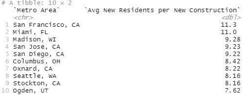
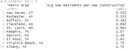
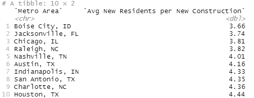
Alright, let's try another tack. What are the NIMBYest and YIMBYest cities in the US, defined by how many new residents there were each year for each new property they built. So if you build 1,000 new properties and your city population grows by 5,000, you should have 5 new residents residents per new construction.
master_df %>%
  select(Metro_Area, year, total_new_construction, absolute_pop_change) %>%
  filter(year<2020) %>%
  filter(absolute_pop_change>0) %>%
  mutate(new_people_per_construction=absolute_pop_change/total_new_construction) %>%
  group_by(Metro_Area) %>%
  summarise(avg_new_people_per_new_construction=mean(new_people_per_construction)) %>%
  arrange(desc(avg_new_people_per_new_construction)) %>%
  rename("Metro Area"="Metro_Area"
         , "Avg New Residents per New Construction"=avg_new_people_per_new_construction) %>%
  slice_head(n=10)

master_df %>%
  select(Metro_Area, year, total_new_construction, absolute_pop_change) %>%
  filter(year<2020) %>%
  filter(absolute_pop_change>0) %>%
  mutate(new_people_per_construction=absolute_pop_change/total_new_construction) %>%
  group_by(Metro_Area) %>%
  summarise(avg_new_people_per_new_construction=mean(new_people_per_construction)) %>%
  arrange(avg_new_people_per_new_construction) %>%
  rename("Metro Area"="Metro_Area"
         , "Avg New Residents per New Construction"=avg_new_people_per_new_construction) %>%
  slice_head(n=10)
Alright, SF makes sense but Miami? Miami is in Florida and Florida isn't super well known for, like, obeying laws. Like, for the Europeans, Florida is where you go when you've got ten years left to live and you want to start a coke habit. And Ohio? Ohio has population growth? That just feels super off. And...Columbus, Ohio is apparently one of the fastest growing Metros in America... (https://www.nbc4i.com/news/local-news/columbus-among-fastest-growing-metropolitan-areas-as-smaller-ohio-areas-shrink/)
At least the failure of the YIMBYest cities makes sense. If your city is kinda shrinking, like Detroit, then you're going to do artificially well on this. Let's do the simplest fix, just looking at those cities that have had at least one year where the population increased by 20,000 people.
master_df %>%
  select(Metro_Area, year, total_new_construction, absolute_pop_change) %>%
  filter(year<2020) %>%
  filter(absolute_pop_change>20000) %>%
  mutate(new_people_per_construction=absolute_pop_change/total_new_construction) %>%
  group_by(Metro_Area) %>%
  summarise(avg_new_people_per_new_construction=mean(new_people_per_construction)) %>%
  arrange(avg_new_people_per_new_construction) %>%
  rename("Metro Area"="Metro_Area"
         , "Avg New Residents per New Construction"=avg_new_people_per_new_construction) %>%
  slice_head(n=10)
Alright, finally something that matches my intuition, at least mostly. Some cities, like Chicago and Indianapolis are probably here more on general size than health but lots of Texas, North Carolina, some Florida, all that matches my intuition.
Regressions
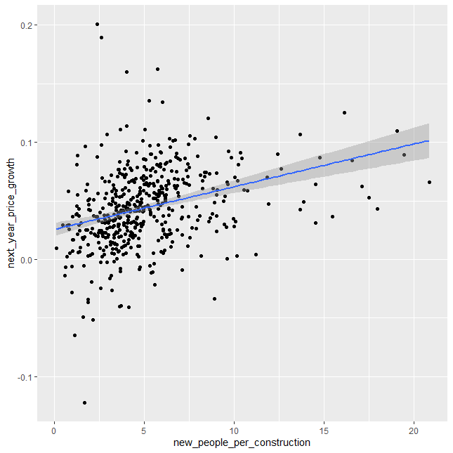
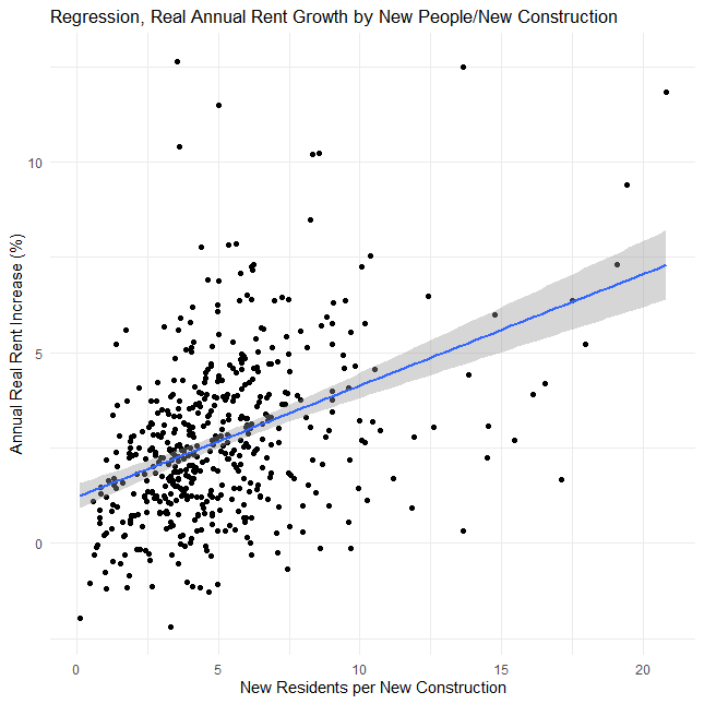
Alright, let's see if we can establish the basic YIMBY relationship, more houses equals lower rent:
test<-master_df %>%
  filter(year<2020) %>%
  filter(absolute_pop_change>0) %>%
  select(year, total_new_construction, absolute_pop_change, real_sale_price, real_rent) %>%
  arrange(year) %>%
  mutate(next_year_price_growth=(lead(real_sale_price)/real_sale_price)-1
         , next_year_rent_growth=(lead(real_rent)/real_rent)-1
         , new_people_per_construction=absolute_pop_change/total_new_construction) %>%
  select(next_year_price_growth, next_year_rent_growth, new_people_per_construction) %>%
  na.omit() %>%
  as.data.frame()

test_price<-test %>%
  select(next_year_price_growth, new_people_per_construction)
ggplot(test_price, aes(new_people_per_construction, next_year_price_growth)) +
  geom_point() +
  geom_smooth(method='lm')

lm(next_year_price_growth~new_people_per_construction, test_price) %>%
  summary()
Alright, and now for rent:
test_rent<-test %>%
  select(next_year_rent_growth, new_people_per_construction) %>%
  mutate(next_year_rent_growth=next_year_rent_growth*100)
ggplot(test_rent, aes(new_people_per_construction, next_year_rent_growth)) +
  geom_point() +
  geom_smooth(method='lm') +
  labs(title="Regression, Real Annual Rent Growth by New People/New Construction"
       , x="New Residents per New Construction", y="Annual Real Rent Increase (%)" ) +
  theme_minimal()

lm(next_year_rent_growth~new_people_per_construction, test_rent) %>%
  summary()
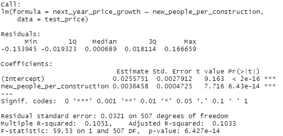
So let's clarify real quick what's being done here. We're doing a really simple linear regression on two factors. First, we take the annual population change from the Census data and divide that by the total amount of new construction from the AEI dataset. Then we determine the annual price change, basically next years average housing price or rent divided by the current price or rent, and then regress or try to predict that price change.
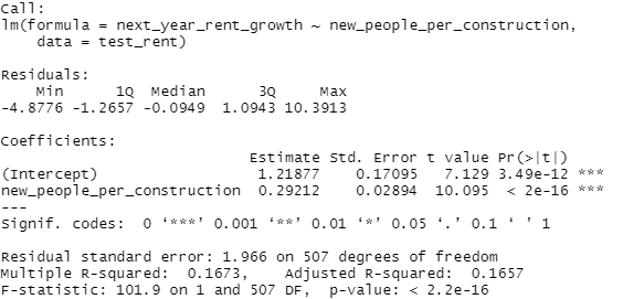
So let's take a look at what we get. which is basically a small but real effect. I mean, this is pretty significant but...that r^2 is pretty low. But what really throws me is the coefficient. Unless I'm grossly misreading this, we've got a pretty clear standard where the zero-intercept, or kinda the base rate, is 1% annual real growth in rent. Now that would require 0 new residents per building, which is kinda abstract, so let's set a real base rate of about 1.3% real annual rent growth if we build one new construction per new resident. That scales at about a quarter of a percent per additional person per property, so at 4 new residents per new construction we'd expect 2% annual rent growth and at 8 new residents per new construction we'd expect about 3% annual rent growth, all else held equal, after inflation.
Now, obviously, real growth varies by a lot more than 1-3% per year, you can see that just from the scatterplot, but this is kinda one of the things I'm getting at, there's a lot more to explaining variations in growth and prices than just new construction. It seems like it should be a big deal, and it is a real effect but it's just not that strong.
And I'll save you some time, I reran these regressions without the outliers and it didn't change the outcome.
A Tale of Two Cities
Alright, instead of a summary let's wrap this up with, bum bum bum, a tale of two cities and a bit of a challenge.
So, here's Austin, arguably the YIMBYest city in America:
master_df %>%
  filter(Metro_Area=="Austin, TX") %>%
  select(year, total_new_construction, absolute_pop_change, Average_Sale_Price) %>%
  rename(Year=year, "New Construction"=total_new_construction, "New People"=absolute_pop_change
         , "Average Home Price"=Average_Sale_Price)
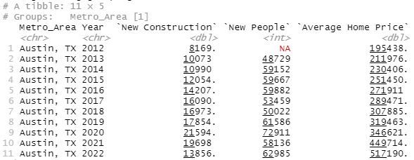
Alright, so what's the YIMBY plan for Austin? The story ain't hard, it's super cool, all the cool people are moving there, wonderful problem to have, and they've handled better than anyone else reasonably could have. They aren't just one of the top cities for new construction, either relative to incoming population or in absolute terms, they almost tripled new construction from ~8k in 2012 to ~21k in 2020. It's hard to ask for somebody to "build, build, build" more than that.
And the result? Even ignoring the Covid housing spike, home prices still went from ~$195k to $319k in 7 years, well over 50%. I mean, it is technically possible to build more, you can go over to Dallas or Houston where they've gone up to 30k-40k per year but that's...that's it, that's the max. And Austin's prices were still going up at 20k new properties/year.
Now take a look at that Covid/post-Covid spike, $319k to $517k in three years. What reasonable path is there to Austin ever returning to that $320k price point? Prices were still going up at 20k new properties, a reasonable spitball of price stability is around 1 new property per 1.5-2 new residents which puts us at 30k to 40k new properties a year for 60k new residents, which is theoretically possible, how much new construction is needed to get prices down by ~40% and how the devil is anybody going to build it?
master_df %>%
  filter(Metro_Area=="San Francisco, CA") %>%
  select(year, total_new_construction, absolute_pop_change, Average_Sale_Price) %>%
  rename(Year=year, "New Construction"=total_new_construction, "New People"=absolute_pop_change
         , "Average Home Price"=Average_Sale_Price)
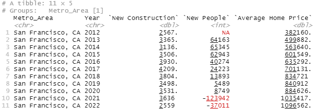
So I'm very sympathetic to YIMBYism in SF, because compared to Austin their new construction numbers are pathetic. Housing prices more than doubled in six years because they were build about a third of what Austin was building despite having a similar influx of people and twice the population.
And I think it's fair to say that SF, at least in the good years, should have been building at least as many new properties as Austin. But what's the story here where SF, which did increase new construction by ~50% from 2012 to 2016, is going to increase new construction by 700-800%? What's an accurate assessment of how much new construction SF actually needs and how the devil are they going to get there.
Because, let's be clear, I'm willing to buy arguments that Austin or San Francisco could stabilize and possibly even reduce prices, in real terms at least, by building near the theoretical Dallas/Houston limit of 30k-40k but Austin at least has a plausible path: they just need to double production, hard but doable, by copying their larger neighbors. What's the story where SF or Oakland or any Bay Area city is going to 10x new construction and start building like Houston? Ignoring the geographical differences, which are big, is SF really going to start regulating like Texas? Texas, where there official state motto is "Don't mess with us" and their unofficial motto is a middle finger to authority? SF is going to do that?
And that's ignoring the far, far deeper damage SF has. You need to drop prices by hundreds of thousands of dollars before normal people, or even tech employees, are going to find it remotely affordable. If SF needs to 10x construction to stabilize prices, how many fricking homes will it take to actually drop the prices and how the devil will SF, of all possible places, achieve rates of building that Texas can't?
Because, if this is just show, if this is just hype to sell people on housing deregulation, promising people it will lead to reasonable rents, which they want, when all it will lead to is price stability, which people need, well that's very much a "hate the game, not the player". Again, I don't want to hate on YIMBYs for overpromising, I hate the system the media game that requires it. Having said that, I'm not confident that YIMBYs know exactly how much they're overpromising.
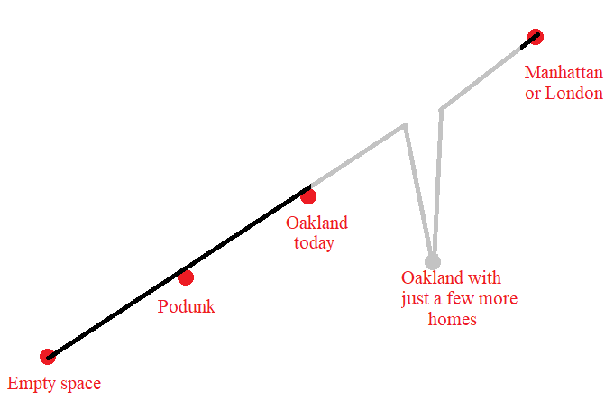
So, in case I'm in danger of fighting a strawman, let me be a bit clear. I'm an ACX fanboy, there was a relatively recent post on housing prices and density, and this graph has stuck with me:
Not because it's right or wrong but because a lot of people, not only commenters but notable economists and YIMBYs all looked at this and were like, "Yeah, this is right, this is what we expect to happen".
Dude, this isn't going to happen. Nobody get big housing decreases. We don't see this anywhere in normal times, only a few places have any price decreases and those are only in inflation adjusted terms and aren't exactly in growing areas. There's no evidence I can find that anyone has built their way to lower housing prices, much less the 30-40% you'd need in, say, SF. Remember, overall we only saw a 20% decrease in housing prices following 2008 (https://en.wikipedia.org/wiki/Subprime_mortgage_crisis). And there's no reasonable path I can see to get there by building.
Nightmares
Finally, let me say this, which I think should stand no matter what your opinion on YIMBY/NIMBY/housing is: this data is a mess and you should generally lower your confidence in all real estate research. Not the dataset, that's actually pretty clean, but I spent easily 80% of my time and code just constantly double checking things like NY having some of the lowest pricing growth, plus the Covid mess, if you can't tell I basically just dropped 2020 on entirely, those Census records are wild and they don't seem to add up right but I've also got, like, 800,000 people moving into NY during Covid but it's the NY MSA so...maybe?
I was constantly struggling with deeply counterintuitive results that I don't trust and what I did show is just what I stared at the numbers long enough to trust but, like:
zip_df<-raw_df[!(is.na(raw_df$ZIP5)), ]
zip_df<-zip_df %>%
  select(ZIP5, orig_y, new_c, price_new_c) %>%
  rename("Zip_Code"=ZIP5, "year"=orig_y) %>%
  group_by(Zip_Code) %>%
  arrange(Zip_Code, year) %>%
  mutate(next_year_price_change=lead(price_new_c)/price_new_c-1) %>%
  filter(year<2020)

summary(lm(next_year_price_change~new_c, zip_df))

zip_df_filter<-zip_df %>%
  filter(Zip_Code %in% c(94027, 02199, 11962, 94957, 33109, 90210, 93108, 94022, 98039, 94024, 11976, 90742, 92662,
                         94970, 94028, 92067, 92657, 92661, 90265, 90272, 10013, 21056, 95070, 10007, 94528, 94010,
                         94920, 89413, 95030, 11932, 90266, 94306, 10282, 92625, 11930, 11959, 94025, 94062, 89402,
                         92651, 91108, 90077, 90212, 94507, 94123, 95014))

summary(lm(next_year_price_change~new_c, zip_df_filter))
zip_df_filter<-zip_df %>%
filter(Zip_Code %in% c(94027, 02199, 11962, 94957, 33109, 90210, 93108, 94022, 98039, 94024, 11976, 90742, 92662,
94970, 94028, 92067, 92657, 92661, 90265, 90272, 10013, 21056, 95070, 10007, 94528, 94010,
94920, 89413, 95030, 11932, 90266, 94306, 10282, 92625, 11930, 11959, 94025, 94062, 89402,
92651, 91108, 90077, 90212, 94507, 94123, 95014))
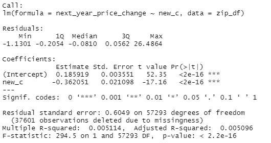
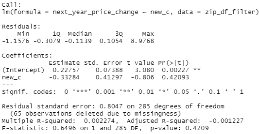
summary(lm(next_year_price_change~new_c, zip_df_filter))So the first regression is just working off the raw zip code data from AEI, regressing the growth in prices of new construction by the % of all sales that were new construction. Just the raw AEI data, almost no opportunity for me to screw it up. Quick 10 minute mental double check that the data is right before moving on to the real analysis. And then, because there's definitely specific zip codes that drive the YIMBY debate, think Manhattan instead of the NY MSA, I decided to go grab a list off Forbes of the most expensive zip codes in the US (https://www.forbes.com/home-improvement/features/most-expensive-zip-codes-us/). And that second regression finds no significant relationship and a smaller effect size and...the whole analysis was like that, I'd run something, there would be something just...deeply unintuitive and, like, once is interesting, a dozen times is maddening. Let me state, bluntly, that I don't trust this result.
So, just a straight up for the people who are really confident in their stance on YIMBY/NIMBY/housing...just be less confident. I'm dramatically less confident in everything because I was constantly confused and triple-checking myself through this analysis and I'm 50% convinced I still got something wrong, I kinda desperately hope someone points out an obvious error in the data section because at least I'd know what the problem was: me. Honestly, my best guess now is that housing prices are some nightmare amalgamation of local income and housing density and age brackets and new construction and interest rates and...if you believe a simple story, well, I dove pretty deep into the data here and it is not simple.
Stuff to do:
If you want more stuff like this, you can read another in depth study I did of family cancellation rates over politics here:
Who cancels and who gets canceled
Table of Contents Intro Goals Overall Risk Methodology notes Political Factors Demographic Factors Life and Satisfaction Factors ML Classification Tree Summary R Code Introduction Alright, so about three months ago Scott Alexander of ACX and SSC fame released his 2022 reader survey which included two questions on cancellations: “Have you cut off any family members …
Or, if you want more posts like this, you could subscribe or share this because, well, it makes a big difference to me:
Or, leave a comment if you liked it, if you have some questions, or best of all, if you find an error in my code.


